Homework 2: BERT Finetuning for Robust Phrasal Chunking
Start on Sep 29 | Due on Oct 15 With grace days Oct 17
Getting Started
If you have already cloned my homework repository nlp-class-hw for
previous homeworks then go into that directory and update the directory:
git pull origin/master
cd nlp-class-hw/bertchunker
If you don’t have that directory anymore then simply clone the repository again:
git clone https://github.com/anoopsarkar/nlp-class-hw.git
Clone your own repository from GitLab if you haven’t done it already:
git clone git@github.sfu.ca:USER/nlpclass-1257-g-GROUP.git
Note that the USER above is the SFU username of the person in
your group that set up the GitLab repository.
Then copy over the contents of the bertchunker directory into your
hw2 directory in your repository.
Set up the virtual environment:
python3.10 -m venv venv
source venv/bin/activate
pip3 install -r requirements.txt
You must use Python 3.10 (or later) for this homework.
Note that if you do not change the requirements then after you have
set up the virtual environment venv you can simply run the following
command to get started with your development for the homework:
source venv/bin/activate
Background
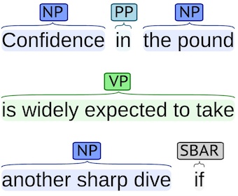
The syntax of a natural language, similar to the syntax of a programming language involves the arrangement of tokens into meaningful groups. Phrasal chunking is the task of finding non-recursive syntactic groups of words. For example, the sentence:
He reckons the current account deficit will narrow to only # 1.8 billion in September .
can be divided into phrasal chunks as follows1:
[NP He] [VP reckons] [NP the current account deficit] [VP will narrow] [PP to] [NP only # 1.8 billion] [PP in] [NP September] .
Data set
The train and test data consist of three columns separated by spaces. Each word has been put on a separate line and there is an empty line after each sentence.
The first column contains the current word, the second column is the part-of-speech tag for that word, and the third column is the chunk tag.
Here is an example of the file format:
He        PRP  B-NP
reckons   VBZ  B-VP
the       DT   B-NP
current   JJ   I-NP
account   NN   I-NP
deficit   NN   I-NP
will      MD   B-VP
narrow    VB   I-VP
to        TO   B-PP
only      RB   B-NP
#         #    I-NP
1.8       CD   I-NP
billion   CD   I-NP
in        IN   B-PP
September NNP  B-NP
.         .    O
The chunk tags contain the name of the chunk type, for example I-NP
for noun phrase words and I-VP for verb phrase words. Most chunk
types have two types of chunk tags, B-CHUNK for the first word of
the chunk and I-CHUNK for each other word in the chunk. See the
Appendix below for a detailed description of the part-of-speech
tags and the chunk tags in this data set. The full set of tags
for this task is in the file data/tagset.txt.
The sequence of labels, B-NP, …, I-NP represents a single
phrasal chunk. For instance, the following sequence of labels:
the       DT   B-NP
current   JJ   I-NP
account   NN   I-NP
deficit   NN   I-NP
gives us the NP phrase:
[NP the current account deficit]
The O chunk tag is used for tokens which are not part of any chunk.
The data set comes from the Conference on Natural Language Learning: CoNLL 2000 shared task2.
There is a helpful program count_sentences.py which allows you
to count how many sentences are in a CoNLL formatted file.
This homework is not just about phrasal chunking but robust phrasal chunking. The input data in dev and test files have been infected with noise so the input to your chunker will look like this:
Rqckwell NNP
, ,
based VBN
in IN
El NNP
Segundo NNP
, ,
Calief. NNP
, ,
is VBZ
an DT
aerospace NN
, ,
electronics NNS
, ,
automotive JJ
and CC
graphics NNS
concern VBP
. .
As you see the words have been infected with noise so
that it contains several spelling mistakes, e.g. Rockwell
is now Rqckwell. The training data is clean and any
model trained on the training data will treat these
noisy words as unknown words.
The input files do not have the output chunk labels
which appear in data/reference/dev.out for input data/input/dev.txt.
Data files
The data files provided are:
data/train.txt.gz– the training data used to train theanswer/default.pymodeldata/input– input filesdev.txtandtest.txtinfected with noisedata/reference/dev.out– the reference output for thedev.txtinput file
Default solution
The default solution is provided in answer/default.py. To use the default
as your solution:
cd answer
cp default.py bertchunker.py
cp default.ipynb bertchunker.ipynb
cd ..
python3 zipout.py
python3 check.py
The default solution will look for the file chunker.pt
in the data directory. If it does not find this file it
will start training on the data/train.txt.gz file. This
will take about 15-20 minutes.
You can also download the chunker.pt model
file
that was trained using default.py.
Please do not commit the file into your git repository as it is moderately large and you can go over your disk quota.
If you have a chunker.pt in the data directory then you can simply run:
python3 answer/default.py > output.txt
And then you can check the score on the dev output file called output.txt by running:
python3 conlleval.py -o output.txt
which produces the following detailed evaluation:
processed 23663 tokens with 11896 phrases; found: 11847 phrases; correct: 10764.
accuracy:  94.01%; (non-O)
accuracy:  94.37%; precision:  90.86%; recall:  90.48%; FB1:  90.67
             ADJP: precision:  79.29%; recall:  69.47%; FB1:  74.06  198
             ADVP: precision:  74.25%; recall:  74.62%; FB1:  74.44  400
            CONJP: precision:  66.67%; recall:  85.71%; FB1:  75.00  9
             INTJ: precision: 100.00%; recall: 100.00%; FB1: 100.00  1
               NP: precision:  90.22%; recall:  91.57%; FB1:  90.89  6330
               PP: precision:  96.80%; recall:  94.31%; FB1:  95.54  2378
              PRT: precision:  80.56%; recall:  64.44%; FB1:  71.60  36
             SBAR: precision:  92.27%; recall:  75.53%; FB1:  83.06  194
               VP: precision:  90.48%; recall:  90.36%; FB1:  90.42  2301
(90.85844517599392, 90.48419636852724, 90.67093459124794)
For this homework we will be scoring your solution based on the FB1 score which is described in detail in the Accuracy section below. However the FB1 score is not the only focus. You can focus on efficiency, model size, experimental comparison with other approaches and many other choices.
Make sure that the command line options are kept as they are in
answer/default.py. You can add to them but you must not delete any
command line options that exist in answer/default.py.
Submitting the default solution without modification will get you zero marks.
The default model
The model used in answer/default.py is a BERT-based Transformer
model that is fine-tuned to predict the phrase chunking tags
for each (sub-word) token. It is trained on the data provided
in data/train.txt.gz which has the ground truth phrase tags
for each token and these sentences are used to fine-tune the
BERT model.
The model structure can be examined using the following code,
assuming that you are in the nlp-class-hw/chunker directory or
if you have the data directory in your current directory with the
training data and the model file:
from default import *
chunker = FinetuneTagger('data/chunker', '.pt', 'distilbert-base-uncased')
print(chunker.model_str())
This prints out the model:
TransformerModel(
  (encoder): DistilBertModel(
    (embeddings): Embeddings(
      (word_embeddings): Embedding(30522, 768, padding_idx=0)
      (position_embeddings): Embedding(512, 768)
      (LayerNorm): LayerNorm((768,), eps=1e-12, elementwise_affine=True)
      (dropout): Dropout(p=0.1, inplace=False)
    )
    (transformer): Transformer(
      (layer): ModuleList(
        (0-5): 6 x TransformerBlock(
          (attention): MultiHeadSelfAttention(
            (dropout): Dropout(p=0.1, inplace=False)
            (q_lin): Linear(in_features=768, out_features=768, bias=True)
            (k_lin): Linear(in_features=768, out_features=768, bias=True)
            (v_lin): Linear(in_features=768, out_features=768, bias=True)
            (out_lin): Linear(in_features=768, out_features=768, bias=True)
          )
          (sa_layer_norm): LayerNorm((768,), eps=1e-12, elementwise_affine=True)
          (ffn): FFN(
            (dropout): Dropout(p=0.1, inplace=False)
            (lin1): Linear(in_features=768, out_features=3072, bias=True)
            (lin2): Linear(in_features=3072, out_features=768, bias=True)
            (activation): GELUActivation()
          )
          (output_layer_norm): LayerNorm((768,), eps=1e-12, elementwise_affine=True)
        )
      )
    )
  )
  (classification_head): Linear(in_features=768, out_features=22, bias=True)
)
Optimizing the above parameters to find the minimum loss on the
training data by gradient descent is done automatically using Pytorch
API calls in answer/default.py.
Hyperparameters
For this homework we will enforce that the base BERT model should not
be changed. Use distilbert-base-uncased as your base BERT model.
You can change the fine-tuning model and parameters as you wish.
Pytorch
You will need to use some Pytorch API calls to solve this homework.
We do not expect you to already know Pytorch in great detail.
The following links will help you get started but you can learn
a lot of the Pytorch basics by understanding default.py and
the process of solving this homework.
Some useful links if you feel lost at the beginning:
Read the source code in default.py in detail.
The Challenge
Your task is to improve the accuracy as much as possible while keeping the hyperparameters used in the default solution for the phrasal chunker. The score is explained in detail in the Accuracy section below. With substantial computational resources and using large pre-trained models (which are beyond the scope of this homework) the state of the art accuracy on this dataset has reached an F1-score above 97 percent (typically by using more information than just the training data available for this task).
However, the numbers from that leaderboard do not apply to the dev and test data in this homework. The dev and test data used here are much more challenging than the standard CoNLL 2000 chunking task because several typos have been introduced into the data (as explained above).
Improving the model
Here are some specific things you can try to improve the accuracy of the fine-tuned model:
- Deal with misspellings in the dev and test data using adversarial training (more details below).
- Use more than the last layer of the Transformer since lower layers of a pre-trained LLM tend to reflect “syntax” while higher levels tend to reflect “semantics” (waving hands profusely).
- Use two different optimizers with different learning rates for the pre-trained encoder layers and the classification head layer. For instance, the classification head parameters might be better learned with an SGD optimizer and a learning rate of \(0.1\).
- Improve the classification head using either:
- multi-layer perceptron (MLP)
- CRF
- mini-Transformer.
You only need to try one or two of these ideas to improve your model for this homework. Dealing with misspellings should be sufficient to get an F-score of higher than 94 on the dev set.
Dealing with Misspellings
A very simple idea for dealing with the misspellings in the dev and test data is to realize that the training data is not similarly noisy. Augmenting the training data with additional noisy examples can help the model handle misspellings at inference time.
For more advanced approach, look into adversarial training as explained in the following paper:
Combating Adversarial Misspellings with Robust Word Recognition. Danish Pruthi, Bhuwan Dhingra, Zachary C. Lipton. ACL 2019.
Improving the classification head
The classification head in default.py is a single linear layer. You could experiment with more expressive feed-forward networks like the following model.
    FFN(
        (dropout): Dropout(p=0.1, inplace=False)
        (lin1): Linear(in_features=768, out_features=3072, bias=True)
        (lin2): Linear(in_features=3072, out_features=768, bias=True)
        (classification_head): Linear(in_features=768, out_features=22, bias=True)
    )
You can experiment with lin1 having more parameters than the input or fewer parameters.
CRF Layer
A Conditional Random Field (CRF) layer can look at consistent labels
(e.g. I tags always follow B tags for the same span, and other
such consistencies) and produce more coherent label sequences.
For an input sequence \(\mathbf{x} = (x_{1}, \ldots, x_{n})\) and a sequence of predictions for the output labels \(\mathbf{y} = (y_{1}, \ldots, y_{n})\) we define a score for the output sequence of labels to be:
$$\textit{score}(\mathbf{x}, \mathbf{y}) = \sum_{i=0}^n C_{y_{i-1},y_{i}} + \sum_{i=1}^n P_{i,y_{i}}$$
The log probability we want to compute is:
$$\textit{log}(g(\mathbf{y} | \mathbf{x})) = \textit{log}(\textit{softmax}_{\mathbf{x}}(\textit{score}(\mathbf{x}, \mathbf{y})))$$
where \(C(y_{i-1},y_{i})\) (or \(C_{i-1}\) for short) is the
transition probability from the labels in the previous time step
to the labels in the current time step \(i\) and \(P_{i,y_{i}}\)
(or \(p(y_{i})\) for one position and \(p(\mathbf{y})\) for the
entire sequence) is the probability of producing label \(y_{i}\)
at time step \(i\). The softmax over the sequence \(\mathbf{x}\)
is computed using tag_space from default.py as follows:
tag_scores = softmax(tag_space, dim=-1) (compare with how
tag_scores is computed in default.py).
Let \(n\) be the length of the sentence aka tag_scores.size(1),
\(B\) be the batch size aka tag_scores.size(0), tagset_size
is the same as tag_scores.size(3), and let \(C_{i-1}\) be the
new variable to store the probability distribution over pairs of
labels (commented out, but called crf_layer in default.py).
You can compute \(\mathbf{y}\) by calling tag_scores.argmax(-1).
Note that because of batching it has two subscripts \(y_{b,i}\)
where \(b\) is each sentence in the batch and \(i\) is the position
in that sentence.
Here is a pseudo-code for the forward function in TransformerModel
which includes a CRF layer that you can add to default.py assuming
tag_space is computed as before (also see the comments in the code).
- For \(b\) in \(B\) and \(i\) in \(n\)
- \(C_{b,i-1} = C(y_{b,i-1})\) (you will need to use
unsqueeze(0)here to create a tensor that can be used to concatenate for all \(b\) values). - \(C_{i-1} = \textit{softmax}([ C_{1,i-1}, \ldots, C_{B,i-1} ])\) (you will need to use
unsqueeze(0)here as well). - \(g_{i} = C_{i-1} + p(y_{i})\) which computes \(\textit{softmax}(\textit{score}(\mathbf{x}, \mathbf{y}))\) for the entire batch and \(p(y_{i})\) is given by
tag_scores[:, i, :].
- \(C_{b,i-1} = C(y_{b,i-1})\) (you will need to use
- return \(g = \textit{log}([ g_{0}, \ldots, g_{n} ])\) (here the concatenation happens for
dim=1which is the sentence length).
Each time the pseudo-code uses \([ v_{1} \ldots v_{q} ]\) for some
tensors \(v_{i}\) it means you should use torch.cat to concatenate
the vectors. You can create an array and append to it for each
\(v_{i}\) and call torch.cat on that array. For the corner case
of \(C_{b,0}\) which is the first token in the sentence for each
\(b\) in the batch you can use \(C_{b,n}\) as the previous time
step since \(C_{b,-1}\) doesn’t exist.
The paper that introduced the use of a CRF layer in neural networks is:
Neural Architectures for Named Entity Recognition. Guillaume Lample, Miguel Ballesteros, Sandeep Subramanian, Kazuya Kawakami, Chris Dyer. NAACL 2016.
Based on the original CRF paper (which you don’t really need to dive into but linked here for completeness):
Conditional Random Fields: Probabilistic Models for Segmenting and Labeling Sequence Data. John Lafferty, Andrew McCallum, Fernando Pereira. ICML 2001.
Some caveats: Implementing a CRF layer is a good exercise since it is complicated to implement and will teach you a lot of PyTorch. However, while many state of the art (SOTA) implementations use a CRF layer, the representation power of a CRF layer is likely superseded by the representations learned using self-attention already in the BERT encoder. Instead of using a CRF layer, it might be easier and more accurate to use multi-head self attention in the classification head.
Required files
You must create the following files:
answer/bertchunker.py– this is your solution to the homework. start by copyingdefault.pyas explained below.answer/bertchunker.ipynb– this is the iPython notebook that will be your write-up for the homework.
Run your solution on the data files
To create the output.zip file for upload to Coursys do:
python3 zipout.py
For more options:
python3 zipout.py -h
Check your accuracy
To check your accuracy on the dev set:
python3 check.py
The output score is the $F_{\beta=1}$ score or FB1 score which is the harmonic mean of the precision and recall computed over all the output phrasal chunks.
python3 check.py -h
In particular use the log file to check your output evaluation:
python3 check.py -l log
The accuracy on data/input/test.txt will not be shown. We will
evaluate your output on the test input after the submission deadline.
Submit your homework on Coursys
Once you are done with your homework submit all the relevant materials to Coursys for evaluation.
Create output.zip
Once you have a working solution in answer/bertchunker.py create
the output.zip for upload to Coursys using:
python3 zipout.py
Create source.zip
To create the source.zip file for upload to Coursys do:
python3 zipsrc.py
You must have the following files or zipsrc.py will complain about it:
answer/bertchunker.py– this is your solution to the homework. start by copyingdefault.pyas explained below.answer/bertchunker.ipynb– this is the iPython notebook that will be your write-up for the homework.
In addition, each group member should write down a short description of what they
did for this homework in answer/README.username.
Upload to Coursys
Go to Homework 2 on Coursys and do a group submission:
- Upload
output.zipandsource.zip - Make sure you have documented your approach in
answer/bertchunker.ipynb. - Check if each group member has a
answer/README.username. - Make sure that your have updated your GitLab repository with your submission source code.
Grading
The grading is split up into the following components:
- dev scores (see Table below)
- test scores (see Table below)
- iPython notebook write-up
- Make sure that you are not using any external data sources in your solution.
- Make sure you have implemented the fine-tuning model improvements yourself without using external libraries.
- Check if each group member has written about what they did in the Python notebook.
Your F-score should be equal to or greater than the score listed for the corresponding marks.
| Score(dev) | Score(test) | Marks | Grade |
| Nan | Nan | 0 | F |
| 90.5 | 82 | 55 | D |
| 91 | 83 | 60 | C- |
| 91.5 | 84 | 65 | C |
| 92 | 85 | 70 | C+ |
| 92.5 | 86 | 75 | B- |
| 93 | 87 | 80 | B |
| 93.5 | 88 | 85 | B+ |
| 94 | 90 | 90 | A- |
| 94.5 | 92 | 95 | A |
| 96 | 95 | 100 | A+ |
The score will be normalized to the marks on Coursys for the dev and test scores.
-
Caveat: If you have a linguistic background, you might find the verb phrases
VPand prepositional phrasesPPare different from what you might be used to. In this task, theVPis a verb and verb modifiers like auxiliaries (were) or modals (might), and thePPsimply contains the preposition. This difference is because of the fact that the chunks are non-recursive (cannot contain other phrases) – we need trees for full syntax. ↩