Homework 1: Word Vectors and the Analogy Task
Start on Sep 15 | Due on Sep 29 With grace days Sep 19
Getting Started
If you have already cloned my homework repository nlp-class-hw for
previous homeworks then go into that directory and update the directory:
git pull origin/main
cd nlp-class-hw/analogy
If you don’t have that directory anymore then simply clone the repository again:
git clone https://github.com/anoopsarkar/nlp-class-hw.git
Clone your own repository from GitLab if you haven’t done it already:
git clone git@github.sfu.ca:USER/nlpclass-1257-g-GROUP.git
Note that the USER above is the SFU username of the person in
your group that set up the GitLab repository.
Then copy over the contents of the analogy directory into your
hw1 directory in your repository.
Set up the virtual environment:
python3 -m venv venv
source venv/bin/activate
pip install -r requirements.txt
Note that if you do not change the requirements then after you have
set up the virtual environment venv you can simply run the following
command to get started with your development for the homework:
source venv/bin/activate
You can also use uv to manage your dependencies.
Background
In this homework we will be exploring the use of word vectors to solve simple analogy tasks.
A word vector is a distributed representation for a word that can be trained via various methods on a word prediction task. A useful word vector is a representation that can capture the usage of the word in context. A properly trained set of word vectors for a language can capture some interesting linguistic relations. These relations can be tested using vector arithmetic to identify aspects of the distributed representation.
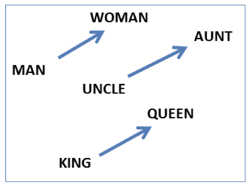
Vector offsets for three word pairs illustrating the gender relation. Figure from https://aclanthology.org/N13-1090.pdf
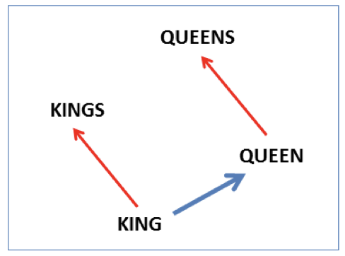
A different projection for the words king, queen showing the singular/plural relation. Figure from https://aclanthology.org/N13-1090.pdf
A common test for word vectors is the aritmetic analogy test. Introducing this test, (Mikolov et al, 2013) proposed to measure the presence of linguistic relations using vector arithmetic.
For two pairs of words (represented by their word vectors) that represent the same linguistic relation, $(a, a^\ast)$ and $(b, b^\ast)$ the test checks for the following approximate equality:
$b + (a^\ast - a) \approx b^\ast$
This approximate equality can be used to solve the analogy task: \(a:a^\ast::b:?\) which is short for saying \(a\) is to \(a^\ast\) as \(b\) is to what?.
This relation can be used to test for various relationships, like the “capital of a country” relationship where if we use (a=France, a*=Paris) and (b=China, b*=?) we expect the above approximate equality to lead us to the vector for b*=Beijing.
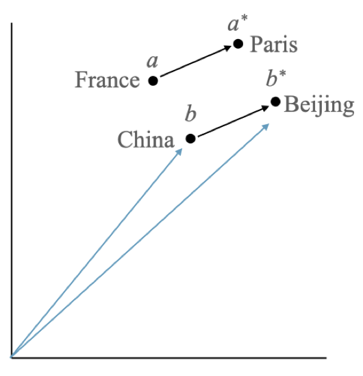
Within pair similarity in the arithmetic analogy test. The vector arithmetic of v(China) + (v(Paris) - v(France)) results in a vector that is close to the vector for the word Beijing. Figure from https://aclanthology.org/2020.conll-1.29.pdf
The Data
The dev and test set for this homework is taken from the Google
word analogy dataset (Mikolov et al., 2013a) was collected for the
following paper on word vectors:
Tomas Mikolov, Kai Chen, Greg Corrado, and Jeffrey Dean. 2013a. Efficient estimation of word representations in vector space. https://arxiv.org/abs/1301.3781
The dataset contains 19544 questions and covers 14 relation types, 7 of which are semantic in nature and 7 are morpho-syntactic (each type is enumerated below). The dataset was created by manually constructing example word-pairs of each relation, and providing all the pairs of word-pairs (within each relation type) as analogy questions.
Default solution
The default solution is provided in answer/default.py. To use the default
as your solution:
cp answer/default.py answer/analogy.py
cp answer/default.ipynb answer/analogy.ipynb
python zipout.py
python check.py
glove-wiki-gigaword-100 model. You must use a 100 dimensional word vector model for this homework. It can be the same glove model that is updated using your code or a different model but make sure you use dimensionality of 100 only.
The default solution will need a network connection to download the glove word embedding model from the gensim servers.
Submitting the default solution without modification will get you zero marks but it provides you with a good start that you can extend towards a better solution.
The overall score reported is the precision score over the entire data set which is described in detail in the Accuracy section below.
The Challenge
Your task is to improve the accuracy as much as possible. The
score is explained in detail in the Accuracy section below. You can
only use the pre-trained word vectors file that has been provided
to you as described in the Default solution section above. You
can modify or train your own word vectors as long as the dimensionality
is kept the same as the default, which is 100d.
Data files
The data files provided are:
data/input– input filesdev.txtandtest.txtdata/reference/dev.out– the reference output for thedev.txtinput filedata/lexicons– lexicon files that contain the word-word relations used for the Baseline method described belowdata/train– training data that can be used to create new lexicons for the Baseline method described below
The lexicon files are as follows:
framenet.txt: from the Framenet projectppdb-xl.txt: from the PPDB projectwordnet-synonyms+.txt: from Wordnetwordnet-synonyms.txt: smaller set of synonyms from Wordnet for use during development
Each file contains a list of words that are assumed to be semantically related to each other. If you consider each ontology as a graph then each line in the above files represents an edge between each pair of words on that line. For example, the line:
faulty incorrect wrong defective
tells that that there is an undirected graph edge representing a
semantic relation between each pair of words on this line, e.g.
faulty-incorrect, faulty-defective, incorrect-defective, and
so on.
Baseline
The baseline method is what you should implement first before you explore additional improvements to improve your score.
First, we will implement retrofitting to combine the information from an ontology (or lexicon) in order to modify the default word vectors.
Retrofitting Word Vectors with Semantic Lexicons
Linguistic relations for words can be found in many semantic lexicons. The most widely used hand-curated semantic lexicon for the English language is the Wordnet ontology.
Of the many semantic relations in Wordnet the most useful to us for this task is that we can identify various groups of words with similar meanings. These groups of words are called synsets (short for synonym sets). However, how do we use these semantic relations to augment the word representations we have in our pre-trained word vectors? This is where retrofitting can be useful. The idea is to use the semantic relations from an ontology like Wordnet and modify or retrofit the word vectors to use that information.
To explain how retrofitting works we need to work with some notation. Let $w_i, w_j$ be words from the vocabulary $V$. Let ${\cal O}$ be an ontology (for example, Wordnet) that encodes semantic relations between words as described in the example above. We represent the ontology as an undirected graph $(V, E)$ with one vertex $v \in V$ for each word type and edges $(w_i, w_j) \in V \subseteq V \times V$ indicating some semantic relationship.
The word vectors for our vocabulary $V$ can be represented by a matrix $\hat{Q}$ which has columns $(\hat{q}_1, \ldots, \hat{q}_n)$ where $|V| = n$ so $\hat{q}_i$ is the word vector for word $w_i$. This matrix of word vectors $\hat{Q}$ has been provided to you as a pre-trained model (the 100 dimensional GloVe word vectors provided above).
The objective of retrofitting is to use the ontology graph ${\cal O}$ in order to learn a matrix $Q = (q_1, \ldots, q_n)$ such that the columns of the matrix $Q$ are close (in vector space) to the word vectors in $\hat{Q} = (\hat{q}_1, \ldots, \hat{q}_n)$ (so $q_i$ is close to $\hat{q}_i$) and at the same time the columns of the matrix $Q$ are close (in vector space) to the word vectors of other words that are adjacent vertices in ${\cal O}$. So if $(w_i, w_j)$ are connected by an edge in the ontology then we want $q_i$ and $q_j$ to be close in vector space. Retrofitting involves combining these two criteria to modify the word vectors for the words in our vocabulary.
For example, the following figure shows how the semantic relations in the ontology (the edges between the white nodes) can be used to learn new retrofitted word vectors (the white nodes). For each word the figures shows a link between the white node for that word (which represents the retrofitted word vectors we wish to learn) and the grey node for the same word (which comes from the pre-trained word vectors).
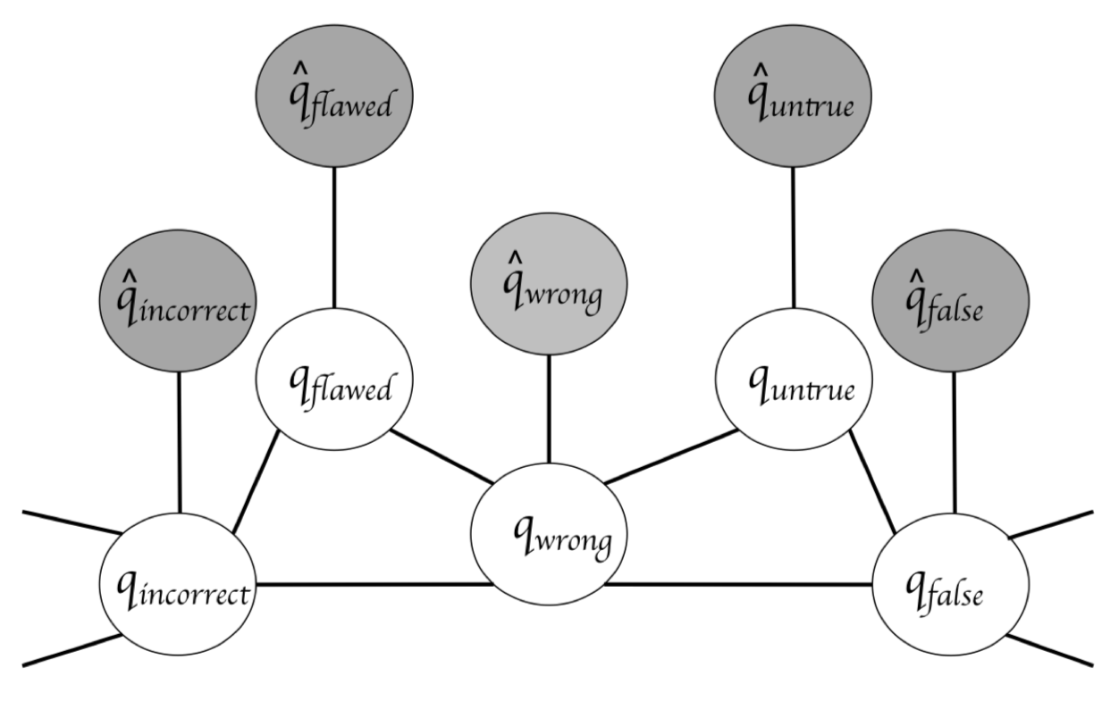
The distance between two word vectors is represented by the Euclidean distance. Our objective function $L$ for finding $Q$ can be written as:
\[L(Q) = \sum_{i=1}^n \left[ \alpha_i || q_i - \hat{q}_i ||^2 + \sum_{(i,j) \in E} \beta_{ij} || q_i - q_j ||^2 \right]\]The algorithm to find $Q$ is as follows:
- Initialize $Q$ to be equal to the vectors in $\hat{Q}$
- For iterations $t = 1 \ldots T$
-
Take the derivative of $L(Q)$ wrt each $q_i$ word vector and assign it to zero to get an update:
\[q_i = \frac{\sum_{j:(i,j) \in E} \beta_{ij} q_j + \alpha_i \hat{q}_i}{\sum_{j:(i,j) \in E} \beta_{ij} + \alpha_i}\]
-
In practice set $T = 10$ which should correspond to changes in Euclidean distance of adjacent vertices of roughly $10^{-2}$. At first, set $\alpha_i = 1$ for all $i$ and $\beta_{ij} = 1$ for all $i,j$. You can try different weighting schemes to see if you get an improvement.
You will have to write your retrofitted word vectors to a file with
the word as first column followed by a space delimited list of 100
floating point numbers. The first line of the file should contain
the total number of words (e.g. 400000) followed by the dimension
of the word vector (e.g. 100). For example, the top two lines of
this file might look like this:
400000 100
the -0.038194 -0.24487 ...97 numbers here... 0.27062
If you are using gensim you can directly load up the retrofitted
text file using KeyedVectors.load_word2vec_format.
Background Reading
For more details read the original paper that introduced the idea of retrofitting word vectors:
Retrofitting Word Vectors to Semantic Lexicons. Faruqui et. al. NAACL 2015.
You can also view the source code that implements retrofitting on GitHub:
You can view the implementation but you must implement the algorithm yourself and apply it to the analogy task.
New Lexicons
You are welcome to design your own model, as long as you have
implemented the Baseline model first. One possible extension is
to create new lexicon files that might help with this particular
set of linguistic relationships. You can use the data in data/train
to create new lexicons.
Required files
You must create the following files in the answer directory:
answer/analogy.py– this is your solution to the homework. start by copyingdefault.pyas explained below.answer/analogy.ipynb– this is the iPython notebook that will be your write-up for the homework.
Run your solution on the data files
To create the output.zip file for upload to Coursys do:
python zipout.py
For more options:
python zipout.py -h
Check your accuracy
To check your accuracy on the dev set:
python check.py
The output score is a precision score comparing your output to the
ground truth in the data/reference directory.
If the output matches the ground truth then we update the count
of true positives $tp$ otherwise we increment the false positives $fp$.
The score for this task is then defined as the
precision score $P$:
For more options:
python check.py -h
In particular use the log file to check your output evaluation:
python check.py -l log
The accuracy on data/input/test.txt will not be shown. We will
evaluate your output on the test input after the submission deadline.
Submit your homework on Coursys
Once you are done with your homework submit all the relevant materials to Coursys for evaluation.
Create output.zip
Once you have a working solution in answer/analogy.py create
the output.zip for upload to Coursys using:
python zipout.py
Create source.zip
To create the source.zip file for upload to Coursys do:
python zipsrc.py
You must have the following files or zipsrc.py will complain about it:
answer/analogy.py– this is your solution to the homework. start by copyingdefault.pyas explained below.answer/analogy.ipynb– this is the iPython notebook that will be your write-up for the homework.
In addition, each group member should write down a short description of what they
did for this homework in answer/README.username.
source.zip or output.zip file uploads to Coursys. Include a script to generate the model files and document it in the answer readme or in the notebook.
Upload to Coursys
Go to Homework 1 on Coursys and do a group submission:
- Upload
output.zipandsource.zip - Make sure your
source.zipmatches your Gitlab repository. - Make sure you have documented your approach in
answer/analogy.ipynb. - Make sure each member of your group has documented their contribution to this homework in
answer/README.usernamewhereusernameis your CSIL/GitLab username.
Grading
The grading is split up into the following components:
- dev scores (see Table below)
- test scores (see Table below)
- iPython notebook write-up
- Make sure that you are not using any external data sources in your solution. You must only use the provided resources: the provided word vector file, optionally the lexicons provided and optionally the training data used to create a new lexicon or new word vector file.
- Make sure you have implemented retrofitting yourself.
- Do not submit the retrofitted word vector file but you should provide a script that produces the retrofitted model used by your homework solution.
- Check if each group member has a
answer/README.username.
Your F-score should be equal to or greater than the score listed for the corresponding marks.
| Score(dev) | Score(test) | Marks | Grade |
| 39.5 | 73.5 | 0 | F |
| 43.5 | 75.5 | 55 | D |
| 46.5 | 77.5 | 60 | C- |
| 49.5 | 79.5 | 65 | C |
| 52.5 | 81.5 | 70 | C+ |
| 55.5 | 83.5 | 75 | B- |
| 58.5 | 85.5 | 80 | B |
| 61.5 | 87.5 | 85 | B+ |
| 64.5 | 89.5 | 90 | A- |
| 68 | 91 | 95 | A |
| 71 | 92 | 100 | A+ |
The score will be normalized to the marks on Coursys for the dev and test scores.
